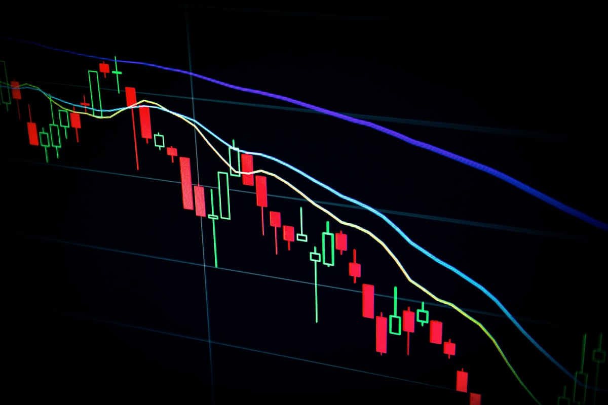
How Python Is Used in Finance: Real Wall Street Use Cases

How Python Is Used in Finance: Real Wall Street Use Cases

When I first heard that investment banks were replacing Excel with Python, I thought it was hype. Then I saw a job listing for "Python Developer — Fixed Income Trading" at a major bank paying $150k+.

Python's adoption in finance is real, deep, and accelerating. This isn't Python as a novelty — it's Python replacing specialized financial software for data analysis, risk modeling, and trading automation.

Here's how Python is actually used in finance, with working code examples.

Why Finance Adopted Python

The finance industry used to run on Excel, Bloomberg Terminal, and proprietary systems. Python displaced Excel for three reasons:

Scale: Python handles millions of rows; Excel breaks at tens of thousands. A risk model running on 10 million trades needs Python.

Reproducibility: Python scripts are versionable with Git. Excel formulas are not.

Libraries: NumPy, pandas, and scikit-learn give financial analysts statistical and ML tools that would take years to build in Excel VBA.

The shift started at hedge funds in the 2010s and has reached investment banks, insurance companies, and fintech startups.

Use Case 1: Financial Data Analysis

The most common Python finance use case: downloading and analyzing market data.

import yfinance as yf
import pandas as pd
import matplotlib.pyplot as plt

# Download stock data
ticker = yf.Ticker("AAPL")
df = ticker.history(period="2y")  # 2 years of daily data

print(df.head())
print(f"\nDate range: {df.index[0].date()} to {df.index[-1].date()}")
print(f"Total trading days: {len(df)}")
print(f"\nPrice stats:\n{df['Close'].describe()}")

pip install yfinance

Comparing Multiple Stocks

def compare_stocks(tickers: list[str], period: str = "1y") -> pd.DataFrame:
    data = {}
    for ticker in tickers:
        stock = yf.Ticker(ticker)
        hist = stock.history(period=period)
        data[ticker] = hist["Close"]
    
    df = pd.DataFrame(data)
    
    # Normalize to 100 (percentage returns from start)
    normalized = df / df.iloc[0] * 100
    
    return normalized

# Compare tech giants
comparison = compare_stocks(["AAPL", "GOOGL", "MSFT", "AMZN"])

plt.figure(figsize=(12, 6))
for col in comparison.columns:
    plt.plot(comparison.index, comparison[col], label=col)

plt.title("Stock Performance (Normalized to 100)")
plt.ylabel("Relative Performance")
plt.legend()
plt.grid(True, alpha=0.3)
plt.tight_layout()
plt.show()

Use Case 2: Returns and Risk Analysis

Calculating Returns

import numpy as np

# Get stock data
aapl = yf.Ticker("AAPL").history(period="2y")

# Daily returns
aapl["Daily_Return"] = aapl["Close"].pct_change()

# Cumulative returns
aapl["Cumulative_Return"] = (1 + aapl["Daily_Return"]).cumprod() - 1

# Summary statistics
print("Return Statistics:")
print(f"  Average daily return: {aapl['Daily_Return'].mean():.4%}")
print(f"  Daily volatility:     {aapl['Daily_Return'].std():.4%}")
print(f"  Annualized return:    {aapl['Daily_Return'].mean() * 252:.2%}")
print(f"  Annualized volatility:{aapl['Daily_Return'].std() * np.sqrt(252):.2%}")
print(f"  Total return:         {aapl['Cumulative_Return'].iloc[-1]:.2%}")

Sharpe Ratio — Risk-Adjusted Return

def sharpe_ratio(returns: pd.Series, risk_free_rate: float = 0.05) -> float:
    """
    Annualized Sharpe ratio.
    risk_free_rate: annual rate (default 5%)
    """
    daily_rf = risk_free_rate / 252
    excess_returns = returns - daily_rf
    return (excess_returns.mean() / excess_returns.std()) * np.sqrt(252)

sharpe = sharpe_ratio(aapl["Daily_Return"].dropna())
print(f"AAPL Sharpe Ratio (2 years): {sharpe:.2f}")

Maximum Drawdown

def max_drawdown(prices: pd.Series) -> float:
    """Maximum peak-to-trough decline."""
    cumulative = (1 + prices.pct_change()).cumprod()
    rolling_max = cumulative.cummax()
    drawdown = (cumulative - rolling_max) / rolling_max
    return drawdown.min()

mdd = max_drawdown(aapl["Close"])
print(f"Maximum Drawdown: {mdd:.2%}")

Use Case 3: Portfolio Analysis

import yfinance as yf
import pandas as pd
import numpy as np

def analyze_portfolio(tickers: list[str], weights: list[float], period: str = "1y") -> dict:
    """Analyze a stock portfolio's performance and risk."""
    
    assert abs(sum(weights) - 1.0) < 1e-9, "Weights must sum to 1"
    
    # Download data
    prices = {}
    for ticker in tickers:
        stock = yf.Ticker(ticker)
        prices[ticker] = stock.history(period=period)["Close"]
    
    price_df = pd.DataFrame(prices).dropna()
    returns = price_df.pct_change().dropna()
    
    # Portfolio returns
    portfolio_returns = (returns * weights).sum(axis=1)
    
    # Metrics
    metrics = {
        "annual_return": portfolio_returns.mean() * 252,
        "annual_volatility": portfolio_returns.std() * np.sqrt(252),
        "sharpe_ratio": sharpe_ratio(portfolio_returns),
        "max_drawdown": max_drawdown(price_df.iloc[:, 0]),  # Simplified
        "total_return": (1 + portfolio_returns).prod() - 1,
    }
    
    # Individual stock contributions
    individual = {}
    for ticker, weight in zip(tickers, weights):
        stock_return = returns[ticker].mean() * 252
        individual[ticker] = {
            "weight": weight,
            "annual_return": stock_return,
            "contribution": weight * stock_return,
        }
    
    return {"portfolio": metrics, "individual": individual}


# Example portfolio
portfolio = analyze_portfolio(
    tickers=["AAPL", "MSFT", "GOOGL", "AMZN", "NVDA"],
    weights=[0.25, 0.25, 0.20, 0.15, 0.15],
    period="1y"
)

print("Portfolio Metrics:")
for metric, value in portfolio["portfolio"].items():
    print(f"  {metric:25}: {value:.2%}")

Use Case 4: Simple Moving Average Strategy

A classic algorithmic trading strategy for educational purposes:

def sma_strategy(ticker: str, short_window: int = 20, long_window: int = 50) -> pd.DataFrame:
    """
    Simple Moving Average crossover strategy.
    Buy when short SMA crosses above long SMA.
    Sell when short SMA crosses below long SMA.
    """
    data = yf.Ticker(ticker).history(period="2y")[["Close"]].copy()
    
    data["SMA_short"] = data["Close"].rolling(window=short_window).mean()
    data["SMA_long"] = data["Close"].rolling(window=long_window).mean()
    
    # Signal: 1 = long, 0 = flat
    data["Signal"] = 0
    data.loc[data["SMA_short"] > data["SMA_long"], "Signal"] = 1
    
    # Position changes
    data["Position"] = data["Signal"].diff()
    
    # Strategy returns
    data["Market_Return"] = data["Close"].pct_change()
    data["Strategy_Return"] = data["Market_Return"] * data["Signal"].shift(1)
    
    # Cumulative
    data["Cumulative_Market"] = (1 + data["Market_Return"]).cumprod()
    data["Cumulative_Strategy"] = (1 + data["Strategy_Return"]).cumprod()
    
    return data

results = sma_strategy("AAPL")
final = results.dropna()

print("SMA Strategy Results for AAPL:")
print(f"Buy & Hold Return:     {final['Cumulative_Market'].iloc[-1] - 1:.2%}")
print(f"Strategy Return:       {final['Cumulative_Strategy'].iloc[-1] - 1:.2%}")

Important disclaimer: Past strategy performance does not predict future returns. This is for educational purposes only — not financial advice.

Use Case 5: Options Pricing (Black-Scholes)

import numpy as np
from scipy.stats import norm

def black_scholes(S, K, T, r, sigma, option_type="call") -> float:
    """
    Black-Scholes option pricing formula.
    S: current stock price
    K: strike price
    T: time to expiration (years)
    r: risk-free interest rate
    sigma: volatility (annualized)
    """
    d1 = (np.log(S / K) + (r + 0.5 * sigma**2) * T) / (sigma * np.sqrt(T))
    d2 = d1 - sigma * np.sqrt(T)
    
    if option_type == "call":
        price = S * norm.cdf(d1) - K * np.exp(-r * T) * norm.cdf(d2)
    else:  # put
        price = K * np.exp(-r * T) * norm.cdf(-d2) - S * norm.cdf(-d1)
    
    return price

# Example: Apple call option
price = black_scholes(
    S=180,      # Current stock price $180
    K=185,      # Strike price $185
    T=30/365,   # 30 days to expiration
    r=0.05,     # 5% risk-free rate
    sigma=0.25, # 25% implied volatility
    option_type="call"
)
print(f"Call option price: ${price:.2f}")

Python Finance Career Paths

Frequently Asked Questions

Is Python used in finance?

Yes — dominant in quantitative finance, risk modeling, trading systems, and financial data analysis at banks, hedge funds, and fintechs.

What Python libraries are used in finance?

pandas, NumPy, yfinance, matplotlib, scikit-learn, statsmodels, Backtrader. QuantLib for derivatives pricing.

Can I use Python for algorithmic trading?

Yes — yfinance for data, Backtrader for backtesting, Alpaca/Interactive Brokers API for live execution. Always backtest thoroughly before live trading.

How do I get financial data in Python?

yfinance for free Yahoo Finance data. Alpha Vantage for free API data. Bloomberg/Refinitiv for professional data.

Final Thoughts

Python's role in finance has moved from novelty to standard practice. The libraries are mature, the community is large, and the career paths are well-defined.

If finance interests you as a Python career path, focus on: pandas mastery, statistical fundamentals (returns, volatility, correlation), and one specialization (data analysis, quant modeling, or fintech development).

The finance + Python combination is among the highest-paying Python career paths. A developer who understands both the code and the financial domain is rare and valued.

For the pandas skills that underpin all financial analysis, our Python data science roadmap covers the data manipulation fundamentals. And for applying machine learning models to financial data, our Python machine learning beginner guide shows the scikit-learn patterns used in quantitative finance.